Examples#
This page will present examples to show the full functionality of otoole. It will
walk through the convert, results, setup, viz and validate
functionality in separate simple use cases.
Note
To follow these examples, clone the Simplicity repository and run all commands
from the simplicity/ directory:
git clone https://github.com/OSeMOSYS/simplicity.git
cd simplicity
Solver Setup#
Objective#
While otoole does not require a solver, these examples will use the free
and open source solvers GLPK, CBC, and HiGHS. Install GLPK (required),
CBC (optional), and HiGHS (optional) to follow along!
1. Install GLPK#
GLPK is a free and open-source linear program solver. Full install instructions can be found on the GLPK Website, however, the abbreviated instructions are shown below
Install on System#
To install GLPK on Linux, run the command:
$ sudo apt-get update
$ sudo apt-get install glpk glpk-utils
To install GLPK on Mac, run the command:
$ brew install glpk
To install GLPK on Windows, follow the instructions on the GLPK Website. Be sure to add GLPK to your environment variables after installation
Install via Anaconda#
Alternatively, if you use Anaconda to manage your Python packages, you can install GLPK via the command:
$ conda install -c conda-forge glpk
Once installed, you should be able to call the glpsol command:
$ glpsol
GLPSOL: GLPK LP/MIP Solver, v4.65
No input problem file specified; try glpsol --help
Tip
See the GLPK Wiki for more information on the glpsol command
2. Install CBC#
CBC is a free and open-source mixed integer linear programming solver. Full install instructions can be found on the CBC website, however, the abbreviated instructions are shown below
Install on System#
To install CBC on Linux, run the command:
$ sudo apt-get install coinor-cbc coinor-libcbc-dev
To install CBC on Mac, run the command:
$ brew install coin-or-tools/coinor/cbc
To install CBC on Windows, follow the install instruction on the CBC website.
Install via Anaconda#
Alternatively, if you use Anaconda to manage your Python packages, you can install CBC via the command:
$ conda install -c conda-forge coincbc
Once installed, you should be able to directly call CBC:
$ cbc
Welcome to the CBC MILP Solver
Version: 2.10.3
Build Date: Mar 24 2020

CoinSolver takes input from arguments ( - switches to stdin)
Enter ? for list of commands or help
Coin:
You can exit the solver by typing quit
3. Install HiGHS#
HiGHS is a free and open-source linear programming (LP), mixed-integer programming (MIP),
and quadratic programming (QP) solver. HiGHS can be run through the command line or through one of their
API interfaces. If you are
using HiGHS through Python, follow the Python installation instructions. If you are running
HiHGS through the command line, follow the Compile From Source or
Precompiled Binary installation instructions.
See also
For further information on installing HiGHS, visit the HiGHS documentation site
Python Install#
In Python, install HiGHS through pip with:
$ pip install highspy
Once installed, you should be able to see highspy in your environment:
$ pip show highspy
Name: highspy
Version: 1.5.3
Summary: Python interface to HiGHS
Home-page: https://github.com/ergo-code/highs
Author:
Author-email:
License: MIT
Location: /home/xxx/.local/lib/python3.10/site-packages
Requires:
Required-by:
Compile from Source#
HiHGS can be installed through CMake for Windows, Mac, or Linux. To do so, first clone the HiHGS repository with the following command:
$ git clone https://github.com/ERGO-Code/HiGHS.git
Next, follow the HiHGS CMake build and install instructions for your operating system. Install instructions for each operating system are described here
Once installed, you should be able to call HiGHS from the command line:
$ highs
Please specify filename in .mps|.lp|.ems format.
Precompiled Binary#
Alternatively from compiling from source, HiHGS can be installed from a pre-compiled binary. To install HiGHS, download a system compatible pre-compiled binary as directed by the HiGHS install documentation.
Extract the binary with the following command on MacOS/Linux:
$ tar -xzf filename.tar.gz
Navigate to the ./bin/ folder and run HiGHS from the command line:
$ ./highs
Tip
To call HiGHS from anywhere in the command line, add the path to the execultable
to your environment variables. For example, if using a bash shell, add the following
to your .bashrc file:
alias highs="/opt/highs/bin/./highs"
export PATH=$PATH:"/opt/highs/bin/"
Once installed, you should be able to call HiGHS from the command line:
$ highs
Please specify filename in .mps|.lp|.ems format.
Input Data Conversion#
Objective#
Convert input data between CSV, Excel, and GNU MathProg data formats.
1. Clone Simplicity#
If not already done so, clone the Simplicity repository:
$ git clone https://github.com/OSeMOSYS/simplicity.git
$ cd simplicity
Note
Further information on the config.yaml file is in the Template Setup section
2. Convert CSV data into MathProg data#
Convert the folder of Simplicity CSVs (data/) into an OSeMOSYS datafile called simplicity.txt:
$ otoole convert csv datafile data simplicity.txt config.yaml
3. Convert MathProg data into Excel Data#
Convert the new Simplicity datafile (simplicity.txt) into Excel data called simplicity.xlsx:
$ otoole convert datafile excel simplicity.txt simplicity.xlsx config.yaml
Tip
Excel workbooks are an easy way for humans to interface with OSeMOSYS data!
4. Convert Excel Data into CSV data#
Convert the new Simplicity excel data (simplicity.xlsx) into a folder of CSV data
called simplicity/. Note that this data will be the exact same as the original CSV data folder (data/):
$ otoole convert excel csv simplicity.xlsx simplicity config.yaml
Process Solutions from Different Solvers#
Objective#
Process solutions from GLPK, CBC, HiGHS, Gurobi, and CPLEX. This example assumes
you have an existing GNU MathProg datafile called simplicity.txt (from the
previous example).
1. Process a solution from GLPK#
Use GLPK to build the model, save the problem as simplicity.glp, solve the model, and
save the solution as simplicity.sol. Use otoole to create a folder of CSV results called results-glpk/.
When processing solutions from GLPK, the model file (*.glp) must also be passed:
$ glpsol -m OSeMOSYS.txt -d simplicity.txt --wglp simplicity.glp --write simplicity.sol

$ otoole results glpk csv simplicity.sol results-glpk datafile simplicity.txt config.yaml --glpk_model simplicity.glp
Note
By default, MathProg OSeMOSYS models will write out folder of CSV results to a results/
directory if solving via GLPK. However, using otoole allows the user to programmatically access results
and control read/write locations
2. Process a solution from CBC#
Use GLPK to build the model and save the problem as simplicity.lp. Use CBC to solve the model and
save the solution as simplicity.sol. Use otoole to create a folder of CSV results called results/ from the solution file:
$ glpsol -m OSeMOSYS.txt -d simplicity.txt --wlp simplicity.lp --check

$ cbc simplicity.lp solve -solu simplicity.sol

$ otoole results cbc csv simplicity.sol results csv data config.yaml
3. Process a solution from HiGHS (CLI)#
Use GLPK to build the model and save the problem as simplicity.lp. Use HiGHS from the command line to solve the model and
save the solution as simplicity.sol. Use otoole to create a folder of CSV results called results/.
HiGHS has the ability to write solutions in a variety of formats; otoole will process the
kSolutionStylePretty solution style. We pass this into the HiGHS solver through an
options file. First, create the options file:
$ touch highs_options.txt
And add the following option to the file:
write_solution_style = 1
Next, we can follow a similar process to processing results from other solvers:
$ glpsol -m OSeMOSYS.txt -d simplicity.txt --wlp simplicity.lp --check

$ highs --model_file simplicity.lp --solution_file simplicity.sol --options_file="highs_options.txt"

$ otoole results highs csv simplicity.sol results csv data config.yaml
Note
Run the following command to see all the options available to pass into highs in the options file:
$ highs --options_file=""
4. Process a solution from HiGHS (Python)#
Use HiGHS Python API to solve a model, and use otoole’s Python API to extract the data into a Python dictionary.
HiGHS can process models in both .mlp and CPLEX .lp format. This example will assume you have a model file
called simplicity.lp already created. This can be created through GLPK following the first command in the previous example.
First, ensure HiGHS is installed in your Python environment:
$ pip install highspy
Next, import highspy and otoole into your Python module:
import highspy
import otoole
Next, use HiGHS to solve the model and write a solution file:
h = highspy.Highs()
h.readModel("simplicity.lp")
h.run()
h.writeSolution("simplicity.sol", 1)
Warning
The HiGHS solution style must be solution style 1 (ie. kSolutionStylePretty)
Finally, use otoole’s otoole.convert.read_results() to read results into a dictionary:
data, defaults = otoole.read_results("config.yaml", "highs", "simplicity.sol", "datafile", "simplicity.txt")
print(data["AnnualEmissions"])

>                           VALUE
> REGION     EMISSION YEAR
> SIMPLICITY CO2      2014  0.335158
>                     2015  0.338832
>                     2016  0.346281
>                     2017  0.355936
...
See also
Using highspy, you are able to extract out detailed solution information as demonstrated
in the HiGHS documentation
here.
5. Process a solution from Gurobi#
Use GLPK to build the model and save the problem as simplicity.lp. Use Gurobi to solve the model and
save the solution as simplicity.sol. Use otoole to create a folder of CSV results called results/ from the solution file:
$ glpsol -m OSeMOSYS.txt -d simplicity.txt --wlp simplicity.lp --check

$ gurobi_cl ResultFile=simplicity.sol simplicity.lp

$ otoole results gurobi csv simplicity.sol results csv data config.yaml
6. Process a solution from CPLEX#
Use GLPK to build the model and save the problem as simplicity.lp. Use CPLEX to solve the model and
save the solution as simplicity.sol. Use otoole to create a folder of CSV results called results/ from the solution file:
$ glpsol -m OSeMOSYS.txt -d simplicity.txt --wlp simplicity.lp --check

$ cplex -c "read simplicity.lp" "optimize" "write simplicity.sol"

$ otoole results cplex csv simplicity.sol results csv data config.yaml
Model Visualization#
Objective#
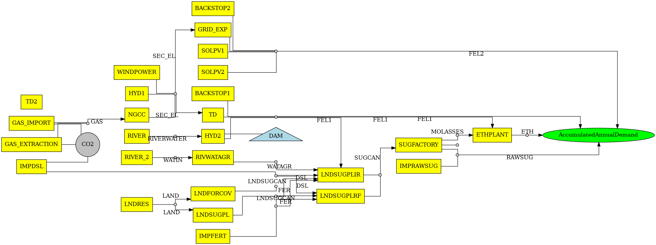
Use otoole to visualize the reference energy system.
1. otoole Visualise#
The visualization functionality of otoole will work with any supported
input data format (csv, datafile, or excel). In this case, we will
use the excel file, simplicity.xlsx, to generate the RES.
Run the following command, where the RES will be saved as the file res.png:
$ otoole viz res excel simplicity.xlsx res.png config.yaml
Warning
If you encounter a graphviz dependency error, install it on your system
following instructions on the Graphviz website. If on Windows,
download the install package from Graphviz.
If on Mac or Linux, or running conda, use one of the following commands:
brew install graphviz       # if on Mac
sudo apt install graphviz   # if on Ubuntu
conda install graphviz      # if using conda
To check that graphviz installed correctly, run dot -V to check the
version:
$ dot -V
dot - graphviz version 2.43.0 (0)
2. View the RES#
Open the newly created file, res.png and the following image should be
displayed
Template Setup#
Objective#
Generate a template configuration file and excel input file to use with
otoole convert commands
1. Create the Configuration File#
Run the following command, to create a template configuration file
called config.yaml:
$ otoole setup config template_config.yaml
2. Create the Template Data CSVs#
otoole will only generate template CSV data, however, we want to input
data in Excel format. Therefore, we will first generate CSV data and convert
it to Excel format:
$ otoole setup csv template_data
3. Add Year Definitions#
Open up the the file template_data/YEARS.csv and add all the years over the model
horizon. For example, if the model horizon is from 2020 to 2050, the
template_data/YEARS.csv file should be formatted as follows:
VALUE |
|---|
2020 |
2021 |
2022 |
… |
2050 |
Note
While this step in not technically required, by filling out the years in
CSV format otoole will pivot all the Excel sheets on these years.
This will save significant formatting time!
4. Convert the CSV Template Data#
Convert the template CSV data into Excel formatted data:
$ otoole convert csv excel template_data template.xlsx template_config.yaml
5. Add Model Data#
There should now be a file called template.xlsx that the user can open and
add data to.
Model Validation#
Note
In this example, we will use a very simple model instead of the Simplicity demonstration model. This way the user does not need to be familiar with the naming conventions of the model.
Objective#
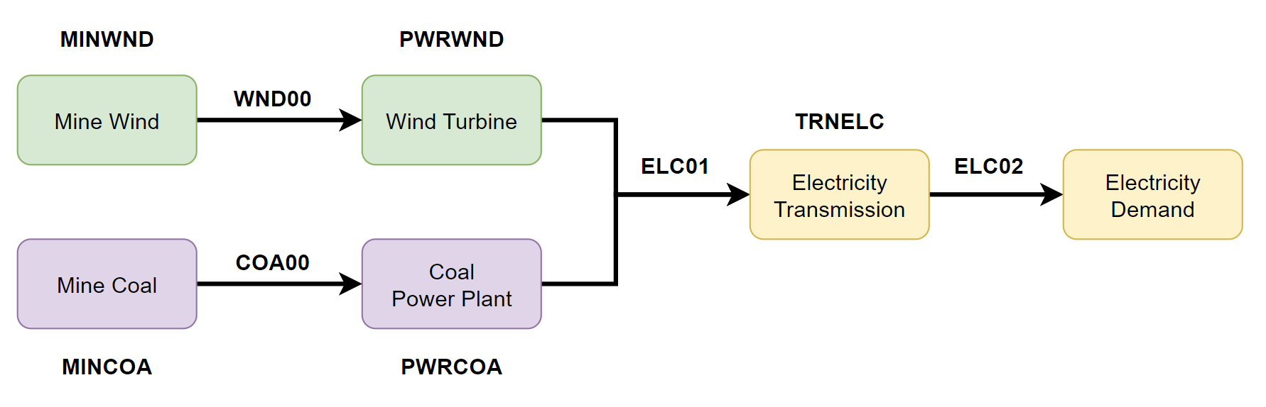
Use otoole to validate an input data file. The model
we are going to validate is shown below, where the fuel and technology
codes are shown in bold face.
1. Download the example datafile#
The MathProg datafile describing this model can be found on the
Example Validation File page. Download the file and save it as data.txt
2. Create the Validation File#
Create a configuration validation yaml file:
# on UNIX
$ touch validate.yaml

# on Windows
> type nul > validate.yaml
3. Create FUEL Codes#
Create the fuel codes and descriptions in the validation configuration file:
codes:
  fuels:
    'WND': Wind
    'COA': Coal
    'ELC': Electricity
  identifiers:
    '00': Primary Resource
    '01': Intermediate
    '02': End Use
4. Create TECHNOLOGY Codes#
Add the technology codes to the validation configuration file. Note that the powerplant types are the same codes as the fuels, so there is no need to redefine these codes:
codes:
  techs:
    'MIN': Mining
    'PWR': Generator
    'TRN': Transmission
5. Create FUEL Schema#
Use the defined codes to create a schema for the fuel codes:
schema:
  FUEL:
  - name: fuel_name
    items:
    - name: type
      valid: fuels
      position: (1, 3)
    - name: identifier
      valid: identifiers
      position: (4, 5)
6. Create TECHNOLOGY Schema#
Use the defined codes to create a schema for the technology codes:
schema:
  TECHNOLOGY:
  - name: technology_name
    items:
    - name: tech
      valid: techs
      position: (1, 3)
    - name: fuel
      valid: fuels
      position: (4, 6)
7. Save changes#
The final validation configuration file for this example will look like:
codes:
  fuels:
    'WND': Wind
    'COA': Coal
    'ELC': Electricity
  identifiers:
    '00': Primary Resource
    '01': Intermediate
    '02': End Use
  techs:
    'MIN': Mining
    'PWR': Generator
    'TRN': Transmission

schema:
  FUEL:
  - name: fuel_name
    items:
    - name: type
      valid: fuels
      position: (1, 3)
    - name: identifier
      valid: identifiers
      position: (4, 5)
  TECHNOLOGY:
  - name: technology_name
    items:
    - name: tech
      valid: techs
      position: (1, 3)
    - name: fuel
      valid: fuels
      position: (4, 6)
8. otoole validate#
Use otoole to validate the input data (can be any of a datafile, csv, or excel)
against the validation configuration file:
$ otoole validate datafile data.txt config.yaml --validate_config validate.yaml

***Beginning validation***

Validating FUEL with fuel_name

^(WND|COA|ELC)(00|01|02)
4 valid names:
WND00, COA00, ELC01, ELC02

Validating TECHNOLOGY with technology_name

^(MIN|PWR|TRN)(WND|COA|ELC)
5 valid names:
MINWND, MINCOA, PWRWND, PWRCOA, TRNELC


***Checking graph structure***
Warning
Do not confuse the user configuration file (config.yaml) and the
validation configuration file (validate.yaml). Both configuration files
are required for validation functionality.
9. Use otoole validate to identify an issue#
In the datafile create a new technology that does not follow the specified schema.
For example, add the value ELC03 to the FUEL set:
set FUEL :=
    WND00
    COA00
    ELC01
    ELC02
    ELC03
Running otoole validate again will flag this improperly named value. Moreover it
will also flag it as an isolated fuel. This means the fuel is unconnected from the model:
$ otoole validate datafile data.txt config.yaml --validate_config validate.yaml

***Beginning validation***

Validating FUEL with fuel_name

^(WND|COA|ELC)(00|01|02)
1 invalid names:
ELC03

4 valid names:
WND00, COA00, ELC01, ELC02

Validating TECHNOLOGY with technology_name

^(MIN|PWR|TRN)(WND|COA|ELC)
5 valid names:
MINWND, MINCOA, PWRWND, PWRCOA, TRNELC


***Checking graph structure***

1 'fuel' nodes are isolated:
    ELC03